The inner working of JPEG

Imagine a world without JPEG… well, actually, I can. These days, we’ve got plenty of more advanced image compression formats—JPEG2000, JPEG-LS, WebP, AVIF, and so on. JPEG could almost be called a relic of the past. It’s tech from the late 80s, yet it’s still everywhere simply because it works well enough and became a standard.

That said, the web is gradually shifting to newer formats like AVIF and WebP. WebP, developed by Google, supports both lossy and lossless compression, and it’s starting to pop up all over the internet. I use WebP on my own site to shrink image sizes while keeping the visual quality pretty much identical to JPEG. In fact, it lets me reduce image sizes by over 10x compared to PNG, which is wild.

But this post isn’t about comparing compression formats. It’s about JPEG—and through it, diving into the core ideas that still show up in modern image compression. So let’s talk about what makes JPEG tick.

Structure of JPEG

JPEG is a standard that outlines the steps for compressing an image—but it doesn’t tell you how to implement them. That’s up to the programmer. It also defines how the compressed image data should be stored, typically in the JFIF format. For this post though, I’m focusing purely on the compression process itself.

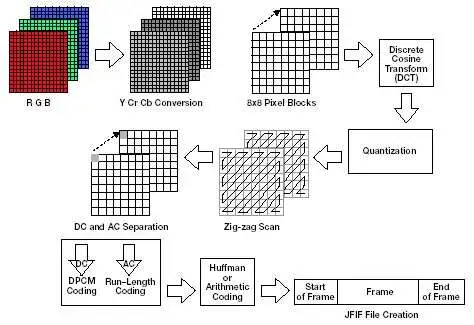
Once you’ve got the raw image pixels, the JPEG algorithm follows five main steps:

1. Convert the RGB image to YUV (or YCbCr) color space.
2. Subsample the U and V (or Cb and Cr) channels.
3. Split each color channel into 8×8 blocks, subtract 128 from each value, and apply the Discrete Cosine Transform (DCT).
4. Quantize the DCT coefficients.
5. Read the data in a zig-zag order and apply Huffman or arithmetic encoding to compress it into binary.

The goal of these steps is to remove as much data from the image while maintaining original quality – that is the old and the new image should look as similar as possible.

The image below sums up how JPEG works:

Reading an image

To keep things simple, I used an uncompressed BMP (Bitmap) image to work with pixel data directly. Most other image formats require extra libraries or more complex logic to read, so I avoided those. BMP gives you the raw RGB pixel values without much fuss.

When reading the image, I skipped anything I didn’t need—no alpha channels or metadata. I just assumed a basic RGB image. While you could handle more complex formats or add alpha support, keep in mind that JPEG isn’t really built for transparency anyway. It doesn’t compress the alpha channel well (or at all), so there’s not much point.

Step 1: Converting to YUV / YCbCr

This is the first step of the JPEG algorithm, and it’s important to understand why it’s done.

Images are made of pixels, and each pixel consists of three primary colors: Red, Green, and Blue—aka RGB. But this format isn’t ideal for JPEG compression, because the information is evenly distributed across all three color channels. That makes it harder to compress efficiently.

The solution? Convert the image to the YUV (or YCbCr) color space.

YUV splits the image into three components:

• Y – the brightness (luma) of the image
• U and V – the color information (chroma)

So what’s the benefit? Our eyes are much more sensitive to brightness changes than to color changes. This means we can compress the color information more aggressively without anyone really noticing. A quick way to see this in action is to compare a grayscale image (just brightness) to one that only has color data with no brightness—the grayscale one still carries most of the detail.

As you can see in the image below, the Y channel (brightness) holds all the details of the image, even though it doesn’t have any color information. On the other hand, the UV channels produce a blurry, hard-to-recognize image.

That’s the core idea behind this step: switching to a format where we can reduce more data without visibly wrecking the image.

Converting between RGB and YUV is lossless and mathematically straightforward. You just apply a simple transformation, and going back to RGB is just the inverse of that.

Here are the formulas used for conversion:

Step 2: UV subsampling

Since the UV (or CbCr) components don’t affect perceived image quality as much as the Y (brightness) component, we can get away with reducing their data. This is done through a simple technique called subsampling.

Subsampling just means taking a small group of values and averaging them into one. For example, if we use 4:1:1 subsampling, it means that for every 4 Y (luma) values, we store only 1 U and 1 V (chroma) value. Other ratios exist, like 4:2:2 or 4:2:0, but 4:1:1 is simple and works really well in practice.

So what does this look like? For the UV channels, we take blocks of 4 pixels and average them into 1. This reduces how much chroma data we store. For example, say an image is 100 pixels wide: without subsampling, that’s 100 Y, 100 U, and 100 V values = 300 total. After 4:1:1 subsampling, we get 100 Y, 25 U, and 25 V = 150 total. That’s half the size with barely any visual difference.

The image below shows how this subsampling process works:

What is DCT?

Now that we’ve done subsampling, it’s time for the real compression magic to start.

The next step in JPEG is something called the Discrete Cosine Transform, or DCT for short. Sounds fancy, but the idea is pretty chill: we’re taking small blocks of pixels (usually 8×8) and breaking them down into their frequency components.

Think of it like this: instead of storing each pixel directly, we ask—“How much of this block looks like a smooth gradient? How much is a sharp edge? How much is just noise?” DCT turns our block of numbers into a bunch of cosine wave patterns, each representing a different “texture” or frequency.

Think of it like this: instead of storing each pixel directly, we ask—“How much of this block looks like a smooth gradient? How much is a sharp edge? How much is just noise?” DCT turns our block of numbers into a bunch of cosine wave patterns, each representing a different “texture” or frequency.

Low frequencies = smooth areas, like the sky or a wall
High frequencies = fine details, edges, or noise

And here’s the trick: our eyes are really good at noticing low-frequency stuff, but not so great at catching the high-frequency bits. So if we drop or shrink some of those high-frequency components, most people won’t even see the difference.

By using DCT, we turn raw pixel data into a format where it’s super easy to throw away stuff that doesn’t matter visually—setting us up for the next step: quantization.

DCT Pre-requisite

Before we can run the Discrete Cosine Transform on the image, we need to prep the data a bit.

First, we split the image into 8×8 blocks. Why 8×8? It’s the sweet spot—big enough to catch useful patterns, but small enough to keep the compression fast and efficient. It also happens to work well with the standard DCT math that JPEG relies on.

If the image dimensions aren’t a multiple of 8 (which is common), we need to pad the image so that it neatly fits into those blocks. The simplest way is to just fill the extra space with zeros. It’s important to also note down how much padding we added (horizontally and vertically), so we can remove it later during decompression.

Next, we need to normalize the pixel values. Normally, pixel intensities range from 0 to 255, but DCT works best when values are centered around zero—i.e., when they oscillate around 0 instead of sitting in a purely positive range.

To fix that, we subtract 128 from each pixel value. This shifts the range to [-128, 127], which is ideal for the transform. (If our image only used the 0–127 range, we’d subtract 64 instead—but most JPEGs span the full 0–255 range, so 128 it is.)

The image below illustrates both the padding and the normalization step—these are the final things we need to handle before applying the DCT.

Step 3: Performing DCT

Now that we’ve got our image split into 8×8 blocks and normalized, it’s time to apply the Discrete Cosine Transform (DCT) to each block.

The main idea behind DCT is to separate useful image information from the less important stuff, like noise or tiny details we probably won’t miss. DCT does this by converting spatial data (pixel values) into frequency data.

In the transformed block, the top-left corner holds the low-frequency components—things like large areas of consistent color or gradual changes. The bottom-right corner holds the high-frequency components—fine details and, often, random noise.

In clean images, most of the important info ends up clustered in the top-left. If the image is noisy, though, you’ll see more high values scattered throughout the block, especially toward the bottom-right. That’s not ideal—but we’ll take care of that in the next step.

Part 4: Quantization

Quantization is where we really start to shrink the data.

The main idea here is to reduce the high-frequency components (which usually represent noise or fine details we don’t really need) and preserve the low-frequency ones (which carry most of the image’s important visual info). This is done using a special 8×8 matrix called the quantization matrix.

This matrix is designed so that its values are small in the top-left corner (low frequencies) and larger in the bottom-right (high frequencies). When we divide our transformed DCT block by this quantization matrix (and round the result), the high-frequency values in the bottom-right mostly turn into zeros. That’s exactly what we want—lots of zeros means easier compression later.

After this step, each 8×8 block is mostly filled with zeros, with just a handful of meaningful values near the top-left.

Here is an example from Wikipedia (DCT coefficient matrix -> quantization matrix -> result):

Part 5.1: Zig-zag reading

With quantization done, the next step is to read the values in a specific pattern—a zig-zag pattern that starts at the top-left (important stuff) and works its way to the bottom-right (mostly zeros).

Why? Because this groups the non-zero values together at the beginning and pushes all the zeros to the end. That makes the next compression step way more efficient.

Part 5.2: DC/AC encoding

In JPEG compression, each 8×8 block is encoded using two kinds of values:

• DC value: the first (top-left) number in the block.
• AC values: the rest of the block, read in zig-zag order.

The actual encoding scheme can vary depending on the JPEG variant, but in the classic approach, these values are compacted using a combination of run-length encoding and simple encoding rules. I won’t go into the exact bitstream structure, but the idea is: more bits are spent on important data, while long stretches of zeros or less useful values are heavily compressed.

Part 5.3: Entropy encoding

Finally, to squeeze things down even more, JPEG uses entropy encoding. This is usually done with Huffman coding or Arithmetic coding.

Most JPEG files stick to predefined Huffman tables, which map commonly seen patterns (like small values or lots of zeros) to short binary codes. It’s a super-efficient way to store the final compressed bitstream.

And just like that—we’ve compressed the image.

And how do we go back?

Going back is pretty straightforward—we just reverse every step we took. Here’s the order:

1. Start with entropy decoding to recover the DC/AC encoded pairs.
2. Decode those DC/AC pairs to get the actual frequency values.
3. Reconstruct the full image blocks from these values.
4. Dequantise by multiplying each value by the quantisation matrix.
5. Run IDCT (inverse DCT) on each 8×8 block to convert back to pixel space.
6. Add 128 to all values to shift the range back from [-128, 127] to [0, 255].
7. Upsample the UV channels if you used chroma subsampling.
8. Convert everything back from YUV to RGB.
9. And finally, write the RGB data to an image file—BMP is a good choice since it’s uncompressed.

Wrapping it up

And that’s basically how JPEG compression works. We strip out what the human eye doesn’t care about, keep what matters, and use clever math to shrink the image without making it look bad. From color space conversion to DCT, quantization, and all the way down to entropy encoding – it’s a chain of smart tricks that works surprisingly well.

Implementing the algorithm isn’t too hard either, especially with a language like Python, where functions like DCT are already built into libraries such as scipy.fftpack or cv2. You just have to understand the steps—and now you do. JPEG is a fascinating algorithm, and it lots of ideas used here apply to other modern image and video compression algorithms.